Automatic differentiation made EaZy

“What I cannot create, I do not understand”, Richard Feynman. I am starting this blog post with a Feynman quote, first and foremost to sound clever, but also because it summarizes well the purpose of EaZyGrad: understanding automatic differentiation at a fundamental level by rebuilding it. Not just a vague idea such as “it is related to the chain rule somehow”, but a useful and reliable mental model of what PyTorch does under the hood when the almighty .backward() is invoked on a tensor.

We will use a simple example throughout this blog post:

import eazygrad as ez

x = ez.tensor([1.0, 2.0, 3.0], requires_grad=True)
y = ez.tensor([0.5, -1.0, 4.0], requires_grad=True)

z = x * y
w = z + x
loss = w.mean()

print(loss)
loss.backward()

print(x.grad)
print(y.grad)

This tiny program already contains some of the core features of a proper deep learning library:

• operations on tensors,

• a reduction to a scalar loss,

• and finally a backward pass that propagates gradients back to the leaf tensors x and y.

The Computation Graph

Leaf tensor is an important concept in an auto-diff engine. To understand it, we first need to explore the concept of a computation graph. At its core, a computation graph is simply a directed graph that records how a value was produced. Each node represents a value, typically a tensor, and each edge represents an operation that transforms one or more inputs into an output. Instead of thinking in terms of “running code line by line”, you can think of the program as building a graph of dependencies between values. Every time you apply an operation such as addition, multiplication, exponentiation, and so on, EaZyGrad creates a corresponding node behind the scenes.

Each node:

• stores the result of the operation,

• keeps references to the parent nodes, its inputs,

• and remembers how it was computed, that is, the operation.

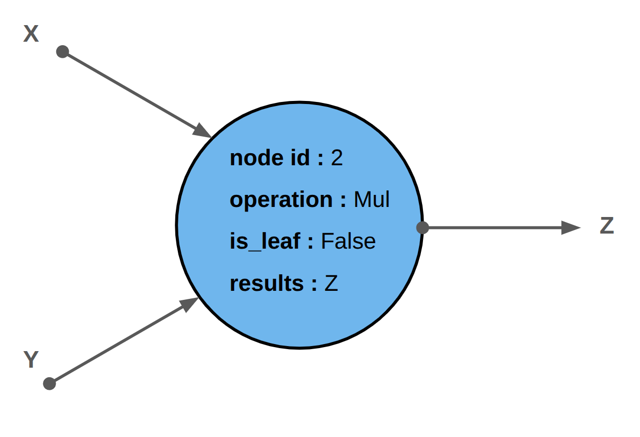
There are three kinds of nodes:

• leaf nodes do not have parent nodes, but they do have children nodes. In the example above, x and y are leaf nodes because they are not the result of any computation.

• root nodes are the exact opposite. They have parent nodes, but no children. In our example, loss is the root node. Backward computation often starts from a scalar root node to produce the gradient that will be backpropagated.

• intermediate nodes sit in the middle. They have both parents and children. In our example, z and w are intermediate nodes.

As a more practical example, when training a neural network, the weights are leaf tensors, the layer activations are intermediate tensors, and the loss is usually the root tensor. Understanding this distinction is important to build a solid mental model of PyTorch. For instance, consider the following PyTorch code:

import torch

a = torch.tensor([1.0, 3.0, 5.0, 7.0], requires_grad=True).reshape(2, 2)
b = torch.tensor([0.5, -1.0], requires_grad=True)

c = a + b
loss = c.mean()
loss.backward()

print(a.grad)

One might expect a.grad to contain the gradient of the tensor a. However, a is not a leaf tensor: it is the result of a computation, namely reshape, which makes it an intermediate tensor. By default, PyTorch frees intermediate gradients after the backward pass. Assuming that a.grad exists would therefore lead to a potentially sneaky bug. EaZyGrad also clears intermediate gradients in the computation graph after the backward pass to save memory. You can see that directly in the tensor operators. Side note: PyTorch exposes the retain_grad() method to prevent intermediate gradient clearing when needed.

Let us now walk through the code of our earlier example, starting with the base _Tensor class, which is essentially a wrapper around a NumPy array. NumPy takes care of the numerical computation, such as addition and multiplication, while EaZyGrad tracks the operations and builds the corresponding computation graph. Here is the _Tensor class in a nutshell:

class _Tensor:
    def __init__(self, array, requires_grad, dtype=None):
        self._array = check.input_array_type(array, dtype)
        self.ndim = self._array.ndim
        self.dtype = self._array.dtype

        if requires_grad and not np.issubdtype(self.dtype, np.floating):
            raise TypeError("Only tensors with floating point dtype can require gradients.")

        self.requires_grad = requires_grad and dag.grad_enable
        self.grad = None
        self.acc_grad = np.float32(0.0)
        self.node_id = None

There are a few important design choices hidden in these few lines.

First, the actual numerical payload lives in self._array, which is just a NumPy array. EaZyGrad does not try to reinvent a numerical kernel library. It delegates the heavy lifting to NumPy and focuses on graph construction and gradient propagation.

Second, requires_grad determines whether the tensor participates in the computation graph. If it is False, the tensor behaves like a plain value container. If it is True, subsequent operations involving that tensor will create graph nodes and record enough information to differentiate later.

Third, there are two gradient-related attributes:

• grad stores the gradient that the user ultimately cares about, for example the gradient of the loss with respect to a model parameter,

• acc_grad is an internal buffer used while gradients are being propagated backward through the graph.

Finally, node_id links the tensor to the node in the computation graph that created it. Leaf tensors start with node_id = None and receive a proper node id when they are registered in the graph. Intermediate tensors are created by operations such as + and *, which immediately allocate a new node and assign that id to the resulting tensor.

Common arithmetic operations are overridden to add computation tracking and build the graph. For instance, the __add__ implementation below is a _Tensor method which computes the result tensor and, if gradients are required, asks the global graph dag to create a node:

def __add__(self, other: _Tensor | float | int) -> _Tensor:
    """
        Overload the '+' operator in python for the _Tensor class.
    """
    ...
    result = _Tensor(self._array + other._array, requires_grad=requires_grad)
    if requires_grad:
        result.node_id = dag.create_node(
            parents_id=[self.node_id, other.node_id],
            operation=operations.Add(),
            result=result,
        )
    return result

The graph itself stores that information in a compact node structure:

class Node:
    def __init__(self, parents_id, operation, result, is_leaf=False):
        self.parents_id = parents_id
        self.operation = operation
        self.result = result
        self.is_leaf = is_leaf

class ComputationGraph:

	def __init__(self) -> None:
		# the computation graph
		# map between node_id and list(parent_id)
		self.dag = {}
		# node id
		self.node_count = -1
		# map between node_id and node
		self.node_map = {}
    
    def _register_node(self, node_id: int, parents_id: list[int | None]) -> None:
		# key : resulting node id
		# values : parents nodes
		self.dag[node_id] = parents_id

    def create_node(self, parents_id: list[int | None], operation: Any, result: Any, is_leaf: bool = False) -> int | None:
		if not self.grad_enable:
			return None
		# Increase node counter for id
		self.node_count += 1
		# Instantiate node
		node = Node(parents_id, operation, result, is_leaf)
		# Store node in a global map 
		self.node_map[self.node_count] = node
		# Register the node in the computation graph
		self._register_node(self.node_count, parents_id)
		return self.node_count

Each intermediate tensor gets a node_id, which is simply the current node_count, that points to the operation that produced it. In other words, the tensor carries a pointer into the computation graph through the node_map variable.

Leaf tensors such as x and y are also registered, but with is_leaf=True and no associated operation. They are the endpoints where gradients are accumulated for the user.

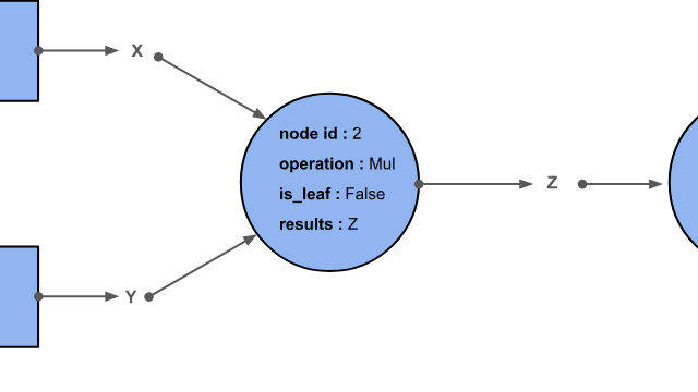
By the end of the forward pass, you have essentially built a fully traceable history of the computation, structured as a graph, like a recording tape. The DAG can be plotted for inspection in EaZyGrad:

loss.plot_dag()

This renders the graph rooted at loss. For our example, the graph contains leaf nodes for x and y, then a multiplication node for z = x * y, then an addition node for w = z + x, and finally a mean reduction for loss. Visualizing the graph is useful because it makes reverse-mode differentiation feel much less magical: .backward() is simply a traversal of that recorded structure.

Playing the tape backward

Right now, we know how the computation graph is created during the forward pass. Let us now walk this process backward. The recording tape analogy was actually not an analogy, but a keyword. PyTorch’s autograd engine implements what is called tape-based reverse mode automatic differentiation. Operations recorded on the tape during the forward pass are replayed in reverse when computing gradients. The process starts from the root node and traverses the graph backward in topological order, meaning each node is visited only after all its children. Calling .backward() on the root tensor fires up this process:

def backward(self, vector: np.ndarray | None = None, retain_graph: bool = False) -> None:
    if vector is None:
        self.acc_grad = np.float32(1.0)
    else:
        self.acc_grad = vector
    dag.backward(self.node_id, retain_graph=retain_graph)

That method on the tensor is intentionally very small. Its job is only to seed the gradient at the root and delegate the real work to the computation graph. If the output is a scalar loss, the seed gradient is 1.0, because:

\[ \frac{\partial L}{\partial L} = 1 \]

The graph then walks backward:

def backward(self, root_node_id: int, retain_graph: bool = False) -> None:
    pending_nodes = []
    heapq.heappush(pending_nodes, -root_node_id)
    while pending_nodes:
        current_node_id = -heapq.heappop(pending_nodes)
        current_node = self.node_map[current_node_id]
        if not current_node.is_leaf:
            grads_inputs = current_node.operation.backward(current_node.result.acc_grad)
            ...
            for parent_id, grad in zip(parent_nodes_id, grads_inputs):
                parent = self.node_map[parent_id]
                grad = ez.check.broadcasted_shape(grad, parent.result)
                parent.result.grad += grad
                parent.result.acc_grad += grad

Conceptually, each step does three things:

1. takes the gradient that has reached the current node (or upstream gradient),

2. applies the local backward rule of the recorded operation using VJPs, see Computing gradients along the way,

3. sends the resulting gradients to the parent nodes (or outgoing gradient).

This is why the operation object is stored during the forward pass. It has stored the context of computation, and therefore knows how to transform an incoming gradient at the output into outgoing gradients for each input. As we will see in section Computing gradients along the way, each operation implements its own local backward rule.

Computing gradients along the way

Let us pause for a minute to summarize what we discussed so far. During the forward pass, each operation performed on tensors is recorded into a computation graph, or a tape. Each node memorizes the context of its creation, namely the input tensors, the operation, and the result, so that the tape can later be played backward. During the backward pass, we start from the root node, usually a scalar loss, and traverse the graph in reverse, applying each operation’s local transformation rule to propagate gradients back to the leaf tensors, where they can then be used by an optimization procedure such as stochastic gradient descent.

The only missing puzzle piece is this: how do we transform an incoming upstream gradient from a child node into outgoing gradients for the parent nodes, based on the operation recorded at the current node? This is the mathematically heavy part, so strap in. If you have a life-threatening allergy to math, you can skip to TL;DR summary in a nutshell for dummies.

Now is the time to talk about the core feature of tape-based reverse mode auto-diff engines: vector-Jacobian products.

But before diving in, let’s briefly recall what a Jacobian is. If we have a vector-valued function

\[ y = f(x), \quad f : \mathbb{R}^m \to \mathbb{R}^n, \]

its Jacobian is the matrix of all partial derivatives:

\[\begin{split} J_f = \begin{bmatrix} \frac{\partial y_1}{\partial x_1} & \cdots & \frac{\partial y_1}{\partial x_m} \\ \vdots & \ddots & \vdots \\ \frac{\partial y_n}{\partial x_1} & \cdots & \frac{\partial y_n}{\partial x_m} \end{bmatrix} \in \mathbb{R}^{n \times m}. \end{split}\]

In practice, differentiation is driven by a scalar objective, usually the loss:

\[ L = g(y). \]

Where \(g\) could be any scalar function, such as a loss function. The gradient that flows backward through the graph from the root is therefore:

\[ v = \frac{\partial L}{\partial x} \]

This vector \(v \in \mathbb{R}^n\) is often called the upstream gradient.

To propagate gradients to \(x\), we apply the chain rule:

\[ \frac{\partial L}{\partial x} = \frac{\partial L}{\partial y} \cdot \frac{\partial y}{\partial x}. \]

Here:

• \(\frac{\partial L}{\partial y} = v\) is the upstream gradient,

• \(\frac{\partial y}{\partial x} = J_f\) is the Jacobian.

So we compute:

\[ \frac{\partial L}{\partial x} = v J_f \]

This is exactly a vector-Jacobian product (VJP). The VJP \(v J_f\) is exactly how the chain rule is applied locally.

A naive implementation of the chain rule would construct the full Jacobian matrix for every operation and multiply it by the incoming gradient. However, this is almost always wasteful.

If an operation maps \(\mathbb{R}^m \to \mathbb{R}^n\), its Jacobian has shape \(n \times m\). In deep learning, these matrices are often enormous, and we rarely need them explicitly. For element-wise operations, Jacobians are diagonal and mostly filled with zeros. In practice, we are not interested in the full Jacobian. We only need its action on an incoming vector. Since \(J_f\) will always have the same structure for a given operation, no matter the inputs, we can derive and hardcode by hand a closed-form equation evaluated at runtime, and avoid to compute the expensive Jacobian \(J_f\). Backpropagation is simply the repeated application of these operation’s specific backward rule, at each node, while traversing the computation graph backward. Lets derive one of such VJP to let this concept sink in.

---

Deriving the VJP for Element-Wise Multiplication

In our running example, the multiplication node is

\[ z = x \odot y \]

where \(x, y, z \in \mathbb{R}^n\), and component-wise:

\[ z_i = x_i y_i \]

---

Step 1 : Jacobian Structure

We begin by asking how each output component depends on each input component:

\[ \frac{\partial z_i}{\partial x_j} \]

Since the multiplication is element-wise, each output \(z_i\) depends only on \(x_i\), not on \(x_j\) for \(j \ne i\). Therefore:

\[\begin{split} \frac{\partial z_i}{\partial x_j} = \begin{cases} y_i & \text{if } i = j \\ 0 & \text{otherwise} \end{cases} \end{split}\]

Thus, the Jacobian of \(z\) with respect to \(x\) is diagonal:

\[\begin{split} J_{z \to x} = \begin{bmatrix} y_1 & 0 & \cdots & 0 \\ 0 & y_2 & \cdots & 0 \\ \vdots & & \ddots & \vdots \\ 0 & 0 & \cdots & y_n \end{bmatrix} \end{split}\]

Similarly:

\[ J_{z \to y} = \operatorname{diag}(x_1, x_2, \dots, x_n) \]

---

Step 2 : Chain Rule Application

Now suppose this multiplication node sits inside a larger computation graph, and we receive an upstream gradient:

\[ v = \frac{\partial L}{\partial z} \]

The chain rule tells us how to propagate this gradient to the inputs:

\[ \frac{\partial L}{\partial x} = \frac{\partial L}{\partial z} \cdot \frac{\partial z}{\partial x} = v J_{z \to x} \]

This is exactly the vector-Jacobian product.

---

Step 3 : Efficient VJP Computation

Multiplying a vector by a diagonal matrix simply scales each component independently:

\[ (v J_{z \to x})_i = v_i y_i \]

So we get:

\[ \frac{\partial L}{\partial x} = v \odot y \]

And similarly:

\[ \frac{\partial L}{\partial y} = v \odot x \]

---

Final VJP Rule

\[ \operatorname{VJP}_{\text{mul}}(v, x, y) = (v \odot y,\; v \odot x) \]

VJPs in action

Let’s recall our running example and apply what we learned to derive the gradient for the two leaf nodes xand y:

\[ z = x \odot y, \qquad w = z + x, \qquad L = \mathrm{mean}(w) \]

where \(\odot\) denotes element-wise multiplication. The graph makes the dependency structure explicit:

• the mean node sends a gradient to \(w\),

• the addition node sends gradients to both \(z\) and \(x\),

• the multiplication node sends gradients to \(x\) and \(y\).

Now let’s run backpropagation step by step and see the VJPs in action.

---

Step 1 : Start from the scalar loss

Since \(L\) is the mean of the components of \(w\),

\[ L = \frac{1}{n}\sum_{i=1}^n w_i \]

the gradient of the loss with respect to \(w\) is:

\[ \frac{\partial L}{\partial w} = \left( \frac{1}{n}, \dots, \frac{1}{n} \right) \]

This is the first upstream gradient injected into the graph by calling .backward() on the scalar loss.

Let us denote it by

\[ v_w = \frac{\partial L}{\partial w}. \]

---

Step 2 : Backprop through the addition node

We now differentiate

\[ w = z + x. \]

For addition, the local backward rule is simple: the upstream gradient is copied unchanged to both parents. In VJP form:

\[ \operatorname{VJP}_{\text{add}}(v_w, z, x) = (v_w,\; v_w) \]

So the addition node sends:

\[ \frac{\partial L}{\partial z} = v_w \qquad\text{and}\qquad \left(\frac{\partial L}{\partial x}\right)_{\text{from add}} = v_w. \]

At this point, \(x\) has already received one gradient contribution, but it is not the final one yet, because \(x\) also influences the loss through the multiplication node.

---

Step 3 : Backprop through the multiplication node

Next we differentiate

\[ z = x \odot y. \]

From the VJP we derived earlier:

\[ \operatorname{VJP}_{\text{mul}}(v_z, x, y) = (v_z \odot y,\; v_z \odot x) \]

with

\[ v_z = \frac{\partial L}{\partial z} = v_w. \]

Therefore, the multiplication node sends:

\[ \left(\frac{\partial L}{\partial x}\right)_{\text{from mul}} = v_w \odot y \]

and

\[ \frac{\partial L}{\partial y} = v_w \odot x. \]

---

Step 4 : Accumulate gradients at shared nodes

The tensor \(x\) has two outgoing paths to the loss:

1. directly through the addition \(w = z + x\),

2. indirectly through the multiplication \(z = x \odot y\).

Because both paths contribute to the final loss, their gradient contributions must be added together:

\[ \frac{\partial L}{\partial x} = \left(\frac{\partial L}{\partial x}\right)_{\text{from add}} + \left(\frac{\partial L}{\partial x}\right)_{\text{from mul}} \]

Substituting the expressions above gives:

\[ \frac{\partial L}{\partial x} = v_w + v_w \odot y \]

and

\[ \frac{\partial L}{\partial y} = v_w \odot x. \]

Since

\[ v_w = \left( \frac{1}{n}, \dots, \frac{1}{n} \right), \]

we can write the final gradients explicitly as:

\[ \frac{\partial L}{\partial x} = \left( \frac{1}{n}, \dots, \frac{1}{n} \right) + \left( \frac{1}{n}, \dots, \frac{1}{n} \right)\odot y \]

and

\[ \frac{\partial L}{\partial y} = \left( \frac{1}{n}, \dots, \frac{1}{n} \right)\odot x. \]

Or, more compactly:

\[ \boxed{ \frac{\partial L}{\partial x} = \frac{1}{n}(1 + y) } \qquad\text{and}\qquad \boxed{ \frac{\partial L}{\partial y} = \frac{1}{n}x } \]

where the operations are understood element-wise.

---

In practice, EaZyGrad implements a VJP for each primitive operations (or computation nodes) : add, mul, matmul, exp, log etc.

class Operation:
    def __init__(self, **kwargs):
        self.context = kwargs
        for ctx in self.context.values():
            if isinstance(ctx, np.ndarray):
                ctx.flags.writeable = False

    def backward(self, grad_output):
        raise NotImplementedError


class Add(Operation):
    def backward(self, grad_output):
        return (grad_output, grad_output)


class Mul(Operation):
    def backward(self, grad_output):
        if "scalar" in self.context:
            scalar = self.context["scalar"]
            return (scalar * grad_output,)

        arr1 = self.context["arr1"]
        arr2 = self.context["arr2"]
        return (arr2 * grad_output, arr1 * grad_output)

Every primitive operation is represented by an Operation object with a single responsibility: given an incoming upstream gradient grad_output, compute the outgoing gradients for its inputs.

The constructor stores the context needed for the backward pass. For multiplication, this means keeping the original input arrays arr1 and arr2, because the local derivatives depend on them:

\[ \frac{\partial (x \odot y)}{\partial x} = y \qquad\text{and}\qquad \frac{\partial (x \odot y)}{\partial y} = x \]

This is why the forward pass must save some data. Once the actual numerical result has been computed, we still need enough information to differentiate that operation later. That saved information is exactly what autograd frameworks call the context. This same pattern repeats for every primitive in the library. Each operation stores just enough context during the forward pass, and later exposes a backward(...) method that computes the local VJP for that operation. It takes the upstream gradient stored in result.acc_grad and returns the VJP for each parent (recall Playing the tape backward). The engine then accumulates those gradients and continues walking backward. More complex operation are interpreted as the composition of multiple primitive operations, such as the mean-squared error operation. In this case, it will chain multiple nodes (substraction \(\to\) squarring \(\to\) mean reduction), each with its own defined VJP. Side-note : instead of composing multiple nodes, one can always fuse these operations into a single node by defining the corresponding VJP. Reducing the number of function call can bring speed up at the cost of a more complex code-base.

Notice also that saved NumPy arrays are marked as non-writeable:

ctx.flags.writeable = False

This is a defensive measure. If the saved context were modified in-place after the forward pass, the backward formulas could silently use corrupted values and produce wrong gradients. By freezing the arrays, EaZyGrad protects the integrity of the recorded tape.

---

TL;DR summary in a nutshell for dummies

Here is the whole story in plain English.

During the forward pass, every tensor operation is recorded in a graph. Each node remembers what operation happened and what values are needed to differentiate it later.

During the backward pass, we start from a scalar value, usually the loss, and move backward through that graph. At each node, we receive the the upstream gradient.

To pass that information to the node’s inputs, we apply the chain rule. Mathematically, this local chain-rule step is a vector-Jacobian product

The important trick is that we do not build the full Jacobian matrix. That would be too expensive and mostly useless. Instead, for each primitive operation, we directly code the formula for the resulting VJP.

For example:

• for addition, the gradient is copied to both inputs,

• for multiplication, the gradient is multiplied by the opposite operand,

• for more complex operations, we use their own specific backward rule.

So in one sentence:

Backpropagation is just the repeated application of local vector-Jacobian products while walking backward through the computation graph.

And in even simpler terms:

Forward pass: compute values.
Backward pass: replay the graph in reverse and distribute contributions using the chain rule.

If this clicked for you, try extending EaZyGrad.

Add new operations, derive their VJPs, or fuse multiple operations into a single node. Each new rule you implement will deepen your intuition for how autodiff systems really work.

Side note : Eager mode

EaZyGrad uses an eager execution model, which applies operations and builds the graph on the fly. In other words, the graph is dynamic and follows the flow of the program. This is flexible, conceptually simple, and very useful because it makes the extremely effective print("here") strategy work when debugging a tensor program. But it is also a significant waste of computing resources:

• it requires rebuilding the graph each time,

• operations are executed as they occur, so no optimization can be done by reordering or fusing them,

• and last but not least, it introduces a large Python overhead. This is why modern Auto-differentiation libraries such as JAX and Tinygrad use Just-in time (JIT) compilation where the graph is created once to trace the flow of computation, optimized by fusing ops or removing python overhead, and then reused for each backward/forward pass. Since Pytorch 2.0, it is also possible to use torch.compile to JIT-compile pytorch code.